HMA Performance Tests
Performance tests are used to relate laboratory mix design to actual field performance. The Hveem (stabilometer) and Marshall (stability and flow) mix design methods use only one or two basic performance tests. Superpave is intended to use a better and more fundamental performance test. However, performance testing is the one area of Superpave yet to be implemented. The performance tests discussed in this section are used by various researchers and organizations to supplement existing Hveem and Marshall tests and as a substitute for the Superpave performance test until it is finalized. This section focuses on laboratory tests; in-place field tests are discussed in Pavement Evaluation.
As with asphalt binder characterization, the challenge in HMA performance testing is to develop physical tests that can satisfactorily characterize key HMA performance parameters and how these parameters change throughout the life of a pavement. These key parameters are:
- Deformation resistance (rutting). A key performance parameter that can depend largely on HMA mix design. Therefore, most performance test efforts are concentrated on deformation resistance prediction.
- Fatigue life. A key performance parameter that depends more on structural design and subgrade support than mix design. Those HMA properties that can influence cracking are largely tested for in Superpave asphalt binder physical tests. Therefore, there is generally less attention paid to developing fatigue life performance tests.
- Tensile strength. Tensile strength can be related to HMA cracking – especially at low temperatures. Those HMA properties that can influence low temperature cracking are largely tested for in Superpave asphalt binder physical tests. Therefore, there is generally less attention paid to developing tensile strength performance tests.
- Stiffness. HMA’s stress-strain relationship, as characterized by elastic or resilient modulus, is an important characteristic. Although the elastic modulus of various HMA mix types is rather well-defined, tests can determine how elastic and resilient modulus varies with temperature. Also, many deformation resistance tests can also determine elastic or resilient modulus.
- Moisture susceptibility. Certain combinations of aggregate and asphalt binder can be susceptible to moisture damage. Several deformation resistance and tensile strength tests can be used to evaluate the moisture susceptibility of a HMA mixture.
Permanent Deformation (Rutting)
Research is ongoing into what type of test can most accurately predict HMA pavement deformation (rutting) There methods currently in use can be broadly categorized as follows:
- ../../../static creep tests. Apply a ../../../static load to a sample and measure how it recovers when the load is removed. Although these tests measure a specimen’s permanent deformation, test results generally do not correlate will with actual in-service pavement rutting measurements.
- Repeated load tests. Apply a repeated load at a constant frequency to a test specimen for many repetitions (often in excess of 1,000) and measure the specimen’s recoverable strain and permanent deformation. Test results correlate with in-service pavement rutting measurements better than ../../../static creep test results.
- Dynamic modulus tests. Apply a repeated load at varying frequencies to a test specimen over a relatively short period of time and measure the specimen’s recoverable strain and permanent deformation. Some dynamic modulus tests are also able to measure the lag between the peak applied stress and the peak resultant strain, which provides insight into a material’s viscous properties. Test results correlate reasonably well with in-service pavement rutting measurements but the test is somewhat involved and difficult to run.
- Empirical tests. Traditional Hveem and Marshall mix design tests. Test results can correlate well with in-service pavement rutting measurements but these tests do not measure any fundamental material parameter.
- Simulative tests. Laboratory wheel-tracking devices. Test results can correlate well with in-service pavement rutting measurements but these tests do not measure any fundamental material parameter.
Each test has been used to successfully predict HMA permanent deformation characteristics however each test has limitations related to equipment complexity, expense, time, variability and relation to fundamental material parameters.
../../../static Creep Tests
A ../../../static creep test (seeFigure 103) is conducted by applying a ../../../static load to an HMA specimen and then measuring the specimen’s permanent deformation after unloading (see Figure 2). This observed permanent deformation is then correlated with rutting potential. A large amount of permanent deformation would correlate to higher rutting potential.
Creep tests have been widely used in the past because of their relative simplicity and availability of equipment. However, ../../../static creep test results do not correlate well with actual in-service pavement rutting (Brown et al., 2001[1]).
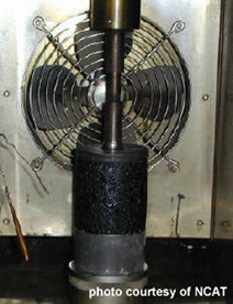 Figure 103: Unconfined ../../../static Creep Test
Unconfined ../../../static Creep Test
The most popular ../../../static creep test, the unconfined ../../../static creep test (also known as the simple creep test or uniaxial creep test), is inexpensive and relatively easy. The test consists of a ../../../static axial stress of 100 kPa (14.5 psi) being applied to a specimen for a period of 1 hour at a temperature of 40°C (104°F). The applied pressure is usually cannot exceed 206.9 kPa (30 psi) and the test temperature usually cannot exceed 40°C (104°F) or the sample may fail prematurely (Brown et al., 2001[1]). Actual pavements are typically exposed to tire pressures of up to 828 kPa (120 psi) and temperatures in excess of 60°C (140°F). Thus, the unconfined test does not closely simulate field conditions (Brown et al., 2001[1]).
Confined ../../../static Creep Test
The confined ../../../static creep test (also known as the triaxial creep test) is similar to the unconfined ../../../static creep test in procedure but uses a confining pressure of about 138 kPa (20 psi), which allows test conditions to more closely match field conditions. Research suggests that the ../../../static confined creep test does a better job of predicting field performance than the ../../../static unconfined creep test (Roberts et al., 1996[2]).
Diametral ../../../static Creep Test
A diametral ../../../static creep test uses a typical HMA test specimen but turning it on its side so that it is loaded in its diametral plane.
Some standard ../../../static creep tests are:
- AASHTO TP 9: Determining the Creep Compliance and Strength of Hot Mix Asphalt (HMA) Using the Indirect Tensile Test Device
Repeated Load Tests
A repeated load test applies a repeated load of fixed magnitude and cycle duration to a cylindrical test specimen (see Figure 3). The specimen’s resilient modulus can be calculated using the its horizontal deformation and an assumed Poisson’s ratio. Cumulative permanent deformation as a function of the number of load cycles is recorded and can be correlated to rutting potential. Tests can be run at different temperatures and varying loads. The load varies is applied in a short pulse followed by a rest period. Repeated load tests are similar in concept to the triaxial resilient modulus test for unconfined soils and aggregates.
Repeated load tests correlate better with actual in-service pavement rutting than ../../../static creep tests (Brown et al., 2001[1]).
Figure 3. Repeated Load Test Schematic
Note: this example is simplified and shows only 6 load repetitions, normally there are conditioning repetitions followed by a series of load repetitions during the test at a determined load level and possibly at different temperatures.
Most often, results from repeated load tests are reported using a cumulative axial strain curve like the one shown in Figure 4. The flow number (FN) is the load cycles number at which tertiary flow begins. Tertiary flow can be differentiated from secondary flow by a marked departure from the linear relationship between cumulative strain and number of cycles in the secondary zone. It is assumed that in tertiary flow, the specimen’s volume remains constant. The flow number (FN) can be correlated with rutting potential.
Figure 4. Repeated Load Test Results Plot
Unconfined Repeated Load Test
The unconfined repeated load test is comparatively more simple to run than the unconfined test because it does not involve any confining pressure or associated equipment. However, like the unconfined creep test, the allowable test loads are significantly less that those experience by in-place pavement.
Confined Repeated Load Test
The confined repeated load test is more complex than the unconfined test due to the required confining pressure but, like the confined creep test, the confining pressure allows test loads to be applied that more accurately reflect loads experienced by in-place pavements.
Diametral Repeated Load Test
A diametral repeated load test uses a typical HMA test specimen but turning it on its side so that it is loaded in its diametral plane. Diametral testing has two critical shortcomings that hinder its ability to determine permanent deformation characteristics (Brown et al., 2001[1]):
- 1. The state of stress is non-uniform and strongly dependent on the shape of the specimen. At high temperature or load, permanent deformation produces changes in the specimen shape that significantly affect both the state of stress and the test measurements.
- 2. During the test, the only relatively uniform state of stress is tension along the vertical diameter of the specimen. All other states of stress are distinctly nonuniform.
Shear Repeated Load Test
The Superpave shear tester (SST), developed for Superpave, can perform a repeated load test in shear. This test, known as the repeated shear at constant height (RSCH) test, applies a repeated haversine (inverted cosine offset by half its amplitude – a continuous haversine wave would look like a sine wave whose negative peak is at zero) shear stress to an axially loaded specimen and records axial and shear deformation as well as axial and shear load. RSCH data have been shown to have high variability (Brown et al., 2001[1]).
Some standard repeated load tests are:
- AASHTO TP 7: Determining the Permanent Deformation and Fatigue Cracking Characteristics of Hot Mix Asphalt (HMA) Using the Superpave Shear Tester (SST) – Procedure F
- AASHTO TP 31: Determining the Resilient Modulus of Bituminous Mixtures by Indirect Tension
- ASTM D 4123: Indirect Tension Test for Resilient Modulus of Bituminous Mixtures
Dynamic Modulus Tests
Dynamic modulus tests apply a repeated axial cyclic load of fixed magnitude and cycle duration to a test specimen (see Figure 1). Test specimens can be tested at different temperatures and three different loading frequencies (commonly 1, 4 and 16 Hz). The applied load varies and is usually applied in a haversine wave (inverted cosine offset by half its amplitude – a continuous haversine wave would look like a sine wave whose negative peak is at zero). Figure 5 is a schematic of a typical dynamic modulus test.
Figure 5. Dynamic Modulus Test Schematic
Dynamic modulus tests differ from the repeated load tests in their loading cycles and frequencies. While repeated load tests apply the same load several thousand times at the same frequency, dynamic modulus tests apply a load over a range of frequencies (usually 1, 4 and 16 Hz) for 30 to 45 seconds (Brown et al., 2001[1]). The dynamic modulus test is more difficult to perform than the repeated load test since a much more accurate deformation measuring system is necessary.
The dynamic modulus test measures a specimen’s stress-strain relationship under a continuous sinusoidal loading. For linear (stress-strain ratio is independent of the loading stress applied) viscoelastic materials this relationship is defined by a complex number called the “complex modulus” (E*) (Witczak et al., 2002[3]) as seen in the equation below:
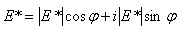
where: E* = complex modulus
= dynamic modulus
φ = phase angle – the angle by which εo lags behind σo.
For a pure elastic material, φ = 0, and the
complex modulus (E*) is equal to the
absolute value, or dynamic modulus. For pure
viscous materials, φ = 90°.
i = imaginary number
The absolute value of the complex modulus, |E*|, is defined as the dynamic modulus and is calculated as follows (Witczak et al., 2002[3]):

where: = dynamic modulus
o = peak stress amplitude
(applied load / sample cross
sectional area)
eo = peak amplitude of recoverable axial strain =
L/L. Either measured directly with strain
gauges or calculated from displacements
measured with linear variable displacement
transducers (LVDTs).
L = gauge length over which the
sample
deformation is measured
= the recoverable portion of the change in sample length
L due to the applied load
The dynamic modulus test can be advantageous because it can measure also measure a specimen’s phase angle (φ), which is the lag between peak stress and peak recoverable strain. The complex modulus, E*, is actually the summation of two components: (1) the storage or elastic modulus component and (2) the loss or viscous modulus. It is an indicator of the viscous properties of the material being evaluated.
Unconfined Dynamic Modulus Test
The unconfined dynamic modulus test is performed by applying an axial haversine load to a cylindrical test specimen. Although the recommend specimen size for the test is 100 mm (4 inch) in diameter by 200 mm (8 inches) high, it may be possible to use smaller specimen heights with success (Brown et al., 2001[1]). Unconfined dynamic modulus tests do not permit the determination of phase angle (φ).
Confined Dynamic Modulus Test
The confined dynamic modulus test is basically the unconfined test with an applied lateral confining pressure. Confined dynamic modulus tests allow for the determination of phase angle (φ). Although the recommend specimen size for the dynamic modulus test is 100 mm (4 inch) in diameter by 200 mm (8 inches) high, it may be possible to use smaller specimen heights with success (Brown et al., 2001[1]). Figure 104 and Figure 105 show a prototype Superpave Simple Performance Test (SPT). The SPT will provide a performance test for the Superpave mix design method.
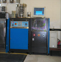 Figure 104: A Prototype Superpave SPT
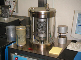 Figure 105: The SPT is a Confined Dynamic Modulus Test
Shear Dynamic Modulus Test
The shear dynamic modulus test is known as the frequency sweep at constant height (FSCH) test. Shear dynamic modulus equations are the same as those discussed above although traditionally the term E* is replace by G* to denote shear dynamic modulus and so ande o are replaced by t0 and g0 to denote shear stress and axial strain respectively. The shear dynamic modulus can be accomplished by two different testing apparatuses:
- 1. Superpave shear tester (SST). The SST FSCH test is a is a constant strain test (as opposed to a constant stress test). Test specimens are 150 mm (6 inches) in diameter and 50 mm (2 inches) tall (see Figure 106). To conduct the test the HMA sample is essentially glued to two plates (see Figure 107 through Figure 109) and then inserted into the SST. Horizontal strain is applied at a range of frequencies (from 10 to 0.1 Hz) using a haversine loading pattern, while the specimen height is maintained constant by compressing or pulling it vertically as required. The SST produces a constant strain of about 100 microstrain (Witczak et al., 2002[3]). The SST is quite expensive and requires a highly trained operator to run thus making it impractical for field use and necessitating further development.
- 2. Field shear tester (FST). The FST FSCH test is a is a constant stress test (as opposed to a constant strain test). The FST is a derivation of the SST and is meant to be less expensive and easier to use. For instance, rather than compressing or pulling the sample to maintain a constant height like the SST, the FST maintains constant specimen height using rigid spacers attached to the specimen ends. Further, the FST shears the specimen in the diametral plane.
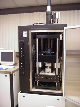 Figure 106: Superpave Shear Tester (SST)
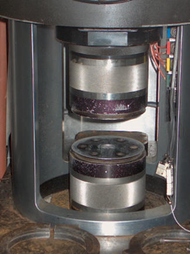 Figure 107: Loading Chamber
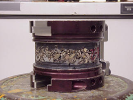 Figure 108: Prepared Sample
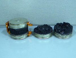 Figure 109: Prepared Sample (left) and Sample After Test.
Standard complex modulus tests are:
- Unconfined dynamic modulus. ASTM D 3497: Dynamic Modulus of Asphalt Mixtures
- Shear dynamic modulus. AASHTO TP 7: Determining the Permanent Deformation and Fatigue Cracking Characteristics of Hot Mix Asphalt (HMA) Using the Simple Shear Test (SST) Device, Procedure E – Frequency Sweep Test at Constant Height.
Empirical Tests
The Hveem stabilometer and cohesiometer and Marshall stability and flow tests are empirical tests used to quantify an HMA’s potential for permanent deformation. They are discussed in their mix design sections.
Simulative Tests – Laboratory Wheel-Tracking Devices
Laboratory wheel-tracking devices (see Video 1/mark>) measure rutting by rolling a small loaded wheel device repeatedly across a prepared HMA specimen. Rutting in the test specimen is then correlated to actual in-service pavement rutting. Laboratory wheel-tracking devices can also be used to make moisture susceptibility and stripping predictions by comparing dry and wet test results Some of these devices are relatively new and some have been used for upwards of 15 years like the Laboratoire Central des Ponts et Chausées (LCPC) wheel tracker – also known as the French Rutting Tester (FRT). Cooley et al. (2000[4]) reviewed U.S. loaded wheel testers and found:
- Results obtained from the wheel tracking devices correlate reasonably well to actual field performance when the in-service loading and environmental conditions of that location are considered.
- Wheel tracking devices can reasonably differentiate between binder performance grades.
- Wheel tracking devices, when properly correlated to a specific site’s traffic and environmental conditions, have the potential to allow the user agency the option of a pass/fail or “go/no go” criteria. The ability of the wheel tracking devices to adequately predict the magnitude of the rutting for a particular pavement has not been determined at this time.
- A device with the capability of conducting wheel-tracking tests in both air and in a submerged state, will offer the user agency the most options of evaluating their materials.
In other words, wheel tracking devices have potential for rut and other measurements but the individual user must be careful to establish laboratory conditions (e.g., load, number of wheel passes, temperature) that produce consistent and accurate correlations with field performance.
Video 1: Asphalt Pavement Analyzer – A Wheel Tracking Device
Fatigue Life
HMA fatigue properties are important because one of the principal modes of HMA pavement failure is fatigue-related cracking, called fatigue cracking. Therefore, an accurate prediction of HMA fatigue properties would be useful in predicting overall pavement life.
Flexural Test
One of the typical ways of estimating in-place HMA fatigue properties is the flexural test (see Figure 110 and Figure 111). The flexural test determines the fatigue life of a small HMA beam specimen (380 mm long x 50 mm thick x 63 mm wide) by subjecting it to repeated flexural bending until failure (see Figure 14). The beam specimen is sawed from either laboratory or field compacted HMA. Results are usually plotted to show cycles to failure vs. applied stress or strain.
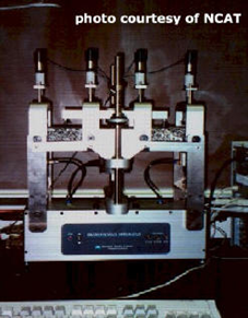 Figure 110: (left). Flexural Testing Device
 Figure 111: (right). Flexural Testing Device
Figure 12: Flexural Test Schematic (click picture to animate)
The standard fatigue test is:
- AASHTO TP 8: Determining the Fatigue Life of Compacted Hot-Mix Asphalt (HMA) Subjected to Repeated Flexural Bending
Tensile Strength
HMA tensile strength is important because it is a good indicator of cracking potential. A high tensile strain at failure indicates that a particular HMA can tolerate higher strains before failing, which means it is more likely to resist cracking than an HMA with a low tensile strain at failure. Additionally, measuring tensile strength before and after water conditioning can give some indication of moisture susceptibility. If the water-conditioned tensile strength is relatively high compared to the dry tensile strength then the HMA can be assumed reasonably moisture resistant. There are two tests typically used to measure HMA tensile strength:
- Indirect tension test
- Thermal cracking test
Indirect Tension Test
The indirect tensile test uses the same testing device as the diametral repeated load test and applies a constant rate of vertical deformation until failure. It is quite similar to the splitting tension test used for PCC.
Standard indirect tension test is a part of the following test:
- AASHTO TP 9: Determining the Creep Compliance and Strength of Hot Mix Asphalt (HMA) Using the Indirect Tensile Test Device
Thermal Cracking Test
The thermal cracking test determines the tensile strength and temperature at fracture of an HMA sample by measuring the tensile load in a specimen which is cooled at a constant rate while being restrained from contraction. The test is terminated when the sample fails by cracking.
The standard thermal cracking test is:
- AASHTO TP 10: Method for Thermal Stress Restrained Specimen Tensile Strength
Stiffness Tests
Stiffness tests are used to determine a HMA’s elastic or resilient modulus. Although these values are fairly well-defined for many different mix types, these tests are still used to verify values, determine values in forensic testing or determine values for new mixtures or at different temperatures. Many repeated load tests can be used to determine resilient modulus as well.
Of particular note, temperature has a profound effect on HMA stiffness. Table 15 shows some typical HMA resilient modulus values at various temperatures. Figure 15 shows that HMA resilient modulus changes by a factor of about 100 for a 56 °C (100 °F) temperature change for “typical” dense-graded HMA mixtures. This can affect HMA performance parameters such as rutting and shoving. This is one reason why the Superpave PG binder grading system accounts for expected service temperatures when specifying an asphalt binder.
Table 15: Typical Resilient Modulus Values for HMA Pavement Materials
| Material | Resilient Modulus (MR) | |
|---|---|---|
| MPa | psi | |
| HMA at 32°F (0 °C) | 14,000 | 2,000,000 |
| HMA at 70°F (21 °C) | 3,500 | 500,000 |
| HMA at 120°F (49 °C) | 150 | 20,000 |
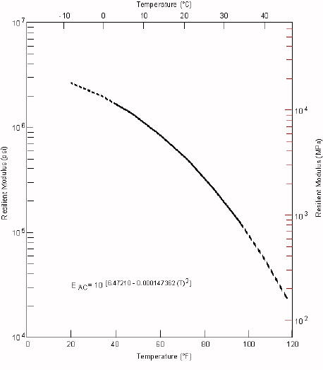 Figure 112: General Stiffness-Temperature Relationship for Dense-Graded
Asphalt Concrete
Figure 112: General Stiffness-Temperature Relationship for Dense-Graded
Asphalt Concrete
Moisture Susceptibility
Numerous tests have been used to evaluate moisture susceptibility of HMA; however, no test to date has attained any wide acceptance (Roberts et al., 1996[2]). In fact, just about any performance test that can be conducted on a wet or submerged sample can be used to evaluate the effect of moisture on HMA by comparing wet and dry sample test results. Superpave recommends the modified Lottman Test as the current most appropriate test and therefore this test will be described.
The modified Lottman test basically compares the indirect tensile strength test results of a dry sample and a sample exposed to water/freezing/thawing. The water sample is subjected to vacuum saturation, an optional freeze cycle, followed by a freeze and a warm-water cycle before being tested for indirect tensile strength (AASHTO, 2000a[5]). Test results are reported as a tensile strength ratio:

where: TSR = tensile strength ratio
S1 = average dry sample tensile strength
S2 = average conditioned sample tensile strength
Generally a minimum TSR of 0.70 is recommended for this method, which should be applied to field-produced rather than laboratory-produced samples (Roberts et al., 1996). For laboratory samples produced in accordance with AASHTO TP 4 (Method for Preparing and Determining the Density of Hot-Mix Asphalt (HMA) Specimens by Means of the Superpave Gyratory Compactor), AASHTO MP 2 (Specification for Superpave Volumetric Mix Design) specifies a minimum TSR of 0.80.
In addition to the modified Lottman test, some state agencies use the Hamburg Wheel Tracking Device (HWTD) to test for moisture susceptibility since the test can be carried out in a warm water bath.
The standard modified Lottman test is:
- AASHTO T 283: Resistance of Compacted Bituminous Mixture to Moisture-Induced Damage